
Introduction
Designing real-time digital signal processing (DSP) pipelines on embedded FPGA hardware requires bridging theoretical signal processing and hardware execution. Before writing VHDL RTL, establishing a bit-true algorithmic model in GNU Octave is essential.
This installment builds the theoretical foundation of our radar pipeline—covering complex I/O baseband representation, Linear Frequency Modulated (LFM) chirps, matched filtering, and a rigorous mathematical breakdown of Processing Gain.
1. Complex Baseband Representation (I & Q Modeling)
In modern digital radar systems, radio frequency (RF) signals are rarely processed directly at carrier frequencies due to sampling rate limitations and ADC bandwidth constraints. Instead, the signal is downconverted to a complex baseband representation consisting of In-phase ($I$) and Quadrature ($Q$) channels:
$$s(t) = I(t) + jQ(t)$$
- Why I/Q? A real-valued sinusoidal signal splits its spectral energy equally between positive and negative frequencies ($f_c$ and $-f_c$), leading to spectral ambiguity. By sampling the signal with two phase-orthogonal local oscillator references ($0^\circ$ for $I$ and $-90^\circ$ for $Q$), we form a complex analytic signal.
- Preserving Phase & Frequency Shift: This complex representation allows the digital signal processor to unambiguously distinguish between positive and negative Doppler frequency shifts (target approaching vs. receding) and preserves instantaneous phase for precise matched filtering.
2. LFM Chirps, Matched Filtering & Simulation Visuals
To achieve high range resolution without requiring impractically high peak transmission power, pulsed radars transmit wideband modulated waveforms—most commonly Linear Frequency Modulated (LFM) chirps. An LFM chirp sweeps its instantaneous frequency linearly across a bandwidth $B$ over a pulse duration $T$:
$$s(t) = \text{rect}\left(\frac{t}{T}\right) \exp\left(j 2\pi \left(f_0 t + \frac{1}{2} k t^2\right)\right)$$
where $k = \frac{B}{T}$ is the frequency modulation slope rate.
According to matched filter theory, the optimal linear filter maximizing output Signal-to-Noise Ratio (SNR) in white Gaussian noise has an impulse response that is the time-reversed, complex conjugate of the transmitted signal:
$$h(t) = s^*(T – t)$$
In digital hardware, complex cross-correlation expands into four parallel real convolutions:
$$(I_{rx} + jQ_{rx}) * (I_{tx} – jQ_{tx}) = (I_{rx}I_{tx} + Q_{rx}Q_{tx}) + j(Q_{rx}I_{tx} – I_{rx}Q_{tx})$$
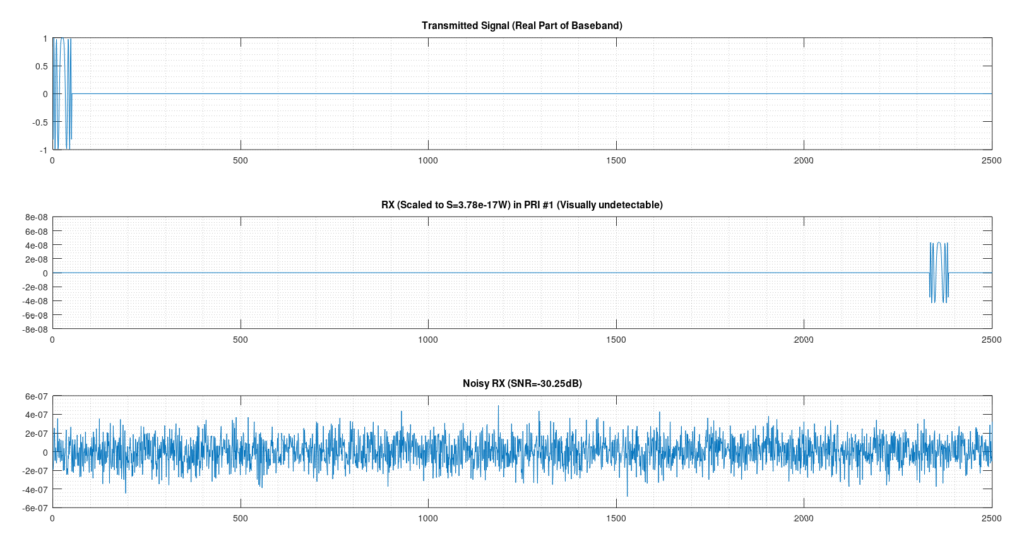
Figure 1: Comparison of the transmitted reference chirp, a clean simulated received echo, and the noise-corrupted received signal ($r(t)$). As illustrated above, single-pulse received echoes are heavily buried beneath thermal noise, rendering raw threshold detection entirely impossible prior to pulse compression.
3. Comprehensive Processing Gain Breakdown
Total processing gain ($G_{\text{total}}$) is achieved through two distinct mechanisms:
- Pulse Compression Gain ($G_{\text{PC}}$): Governed by the Time-Bandwidth Product ($BT$). For a bandwidth $B = 2\text{ MHz}$ and pulse duration $T = 50\ \mu\text{s}$:
$$BT = (2 \times 10^6\text{ Hz}) \times (50 \times 10^{-6}\text{ s}) = 100$$
$$G_{\text{PC(dB)}} = 10 \log_{10}(100) = 20\text{ dB}$$ - Coherent Integration Gain ($G_{\text{coh}}$): Integrating $N = 8$ successive Pulse Repetition Intervals (PRIs) sums signal voltage linearly ($N$) while noise power adds incoherently ($N$), yielding a power SNR gain of:
$$G_{\text{coh(dB)}} = 10 \log_{10}(8) \approx 9.03\text{ dB}$$ - Total System Gain:
$$G_{\text{total(dB)}} = 20\text{ dB} + 9.03\text{ dB} = 29.03\text{ dB}$$
4. Radar Range Equation & Octave Simulation Results
Propagation physics are modeled via the radar range equation, where received power $P_r$ drops off inversely with the fourth power of target range $R$:
$$P_r = \frac{P_t G^2 \lambda^2 \sigma}{(4\pi)^3 R^4 \cdot L}$$
In our simulation framework (Correlation.m), the target is placed at sample index 2333, corresponding to a two-way propagation distance of:
$$R = \frac{c \cdot \tau_{\text{prop}}}{2} \approx 6999\text{ meters}$$
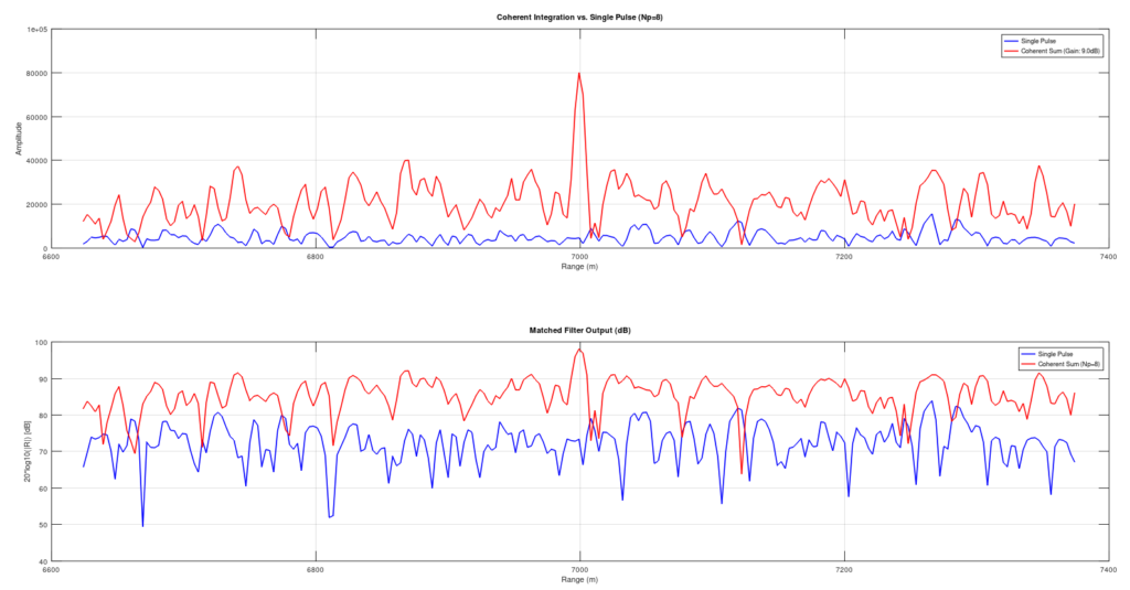
Figure 2: Octave simulation output showing the absolute magnitude of the matched filter response after 8-pulse coherent integration. The noise floor is suppressed, resulting in a sharp, unambiguous detection peak precisely at sample index 2333.
Summary & Next Steps
By establishing the mathematical framework—spanning complex I/Q baseband conversion, LFM chirp compression, and quantitative processing gain calculations—we generate our bit-true golden reference dataset (golden_ref_vector.dat).
In the upcoming hardware implementation post, we transition directly from these Octave models to cycle-accurate VHDL on the Zynq-7000 FPGA, examining time-division folded FIRs, FIFO latency management, and 250 MHz timing closure.
GitHub Repository:
This Link – Stores GNU Octave simulation scripts and VHDL implementation files.
References
- Radar Tutorial: Comprehensive theoretical foundations on pulse compression, matched filtering, and radar range equations. Available at radartutorial.eu.
- Skolnik, Merrill I. Introduction to Radar Systems, 3rd Edition, McGraw-Hill.
Leave a Reply